Fastai Deep Learning Notes
Deep Learning Notes
My Notes based on 2019 FastAI course. The code mentioned below will not work on fastai latest version. However the general information mentioned below is valid.
General stuff
-
Jupyter notebook – Installed through Anaconda. But there are various other ways.
-
Google Collab - https://colab.research.google.com/notebooks/welcome.ipynb - recent=true
-
Use GPU while running the code.
-
GPUs are good at running similar code (in this case mathematical models) multiple times and hence are necessary. CPUs can’t handle or are slow.
-
Pytorch, TensorFlow, FastAI, numpy, pandas, matplotlib etc are all Python libraries. Some are deep learning specific and some are math specific.
-
Data is stored on google compute VM (Collab’s backend) by default. However we can store on Google Drive and access it from within python code.
-
Custom Data can be used and external links (google drive, dropbox etc) will be needed for any proper usage of programs (see lesson 2 notebook in google drive of <emailmanjunathrg@gmail.com)>
-
Visual Studio Code can be used to browse through fastai or pytorch classes and understand the library code.
-
Render can be used to deploy web apps; Google Compute Engine is another option.
-
Further reading - Different types of Models (Resnet, Inception, VGGNet, AlexNet etc)
Below lines of code are needed when running notebooks using FastAI. Few are for Google Drive, Library Reloads, Ignore Pytorch related warnings, plotting inline in the notebook
!curl -s https://course.fast.ai/setup/colab bash %reload_ext autoreload
%autoreload 2
%matplotlib inline
import warnings
warnings.filterwarnings(“ignore”, category=UserWarning, module=”torch.nn.functional”)
from google.colab import drive
drive.mount(‘/content/gdrive’, force_remount=True)
root_dir = ”/content/gdrive/My Drive/”
base_dir = root_dir + ’fastai-v3/’
Below is a javascript to download URLs from google search images into a csv file. I think it should work with any google search result.
Press CtrlShiftJ in Windows/Linux and CmdOptJ in Mac and paste below and enter. A csv file should get downloaded.
urls = Array.from(document.querySelectorAll(‘.rg_di .rg_meta’)).map(el=>JSON.parse(el.textContent).ou);
window.open(‘data:text/csv;charset=utf-8,’ + escape(urls.join(‘\n’)));
General Process for Training a Model
Below is a general flow for train a model. This is very general and at a high level.
There can be lots of variations and other steps in between and after.
Get the data with data (like images) and labels. Example command below
Labels can be present in various ways and below command/process will need to be changed accordingly.
data = ImageDataBunch.from_folder(path, train=”.”, valid_pct=0.2,
ds_tfms=get_transforms(), size=224, num_workers=4).normalize(imagenet_stats)
Train the model using a CNN (convolutional neural network)
learn = cnn_learner(data, models.resnet34, metrics=error_rate)
Fit the data to the curve correctly using appropriate number of epochs
learn.fit_one_cycle(4)
You can interpret the data after this. You can plot confusion matrix or most confused output also.
interp = ClassificationInterpretation.from_learner(learn)
interp.plot_confusion_matrix()
Once you think the model has learnt, you can export the model so that it can be used in an application. This will create a file named ‘export.pkl’ in the directory where we were working that contains everything we need to deploy our model (the model, the weights but also some metadata like the classes or the transforms/normalization used).
learn.export()
This export file can be used to deploy on Render.com or Google Compute etc.
Example -
https://github.com/mrg-ai/SouthIndianSnackClassifier
**
DataBlock API**
In the previous section, we used ImageDataBunch.from_folder method to get the “data” which was then passed to a Learner. This was a factory method from FastAI library. It does quite a few things in the backend and also makes some decisions.
We cannot use Factory methods all the time. We will go through the steps that happen in these type of Factory methods and understand the flow. Then we can use those classes and we can have more control. This will also help in understanding what happens to the data before we send it to a learner. Some of these are Pytorch Classes i.e. Dataset, Dataloader and Databunch is a FastAI class
Dataset – This is the first step in getting the data. An object (like image) and its label(s) form a dataset.
Dataloader – A dataset is not enough to train a model. Batches of datasets need to be sent to the model. For creating these batches, we use a Dataloader.
Databunch – It still isn’t enough to train a model, because we’ve got no way to validate the model. If all we have is a training set, then we have no way to know how we’re doing. We need a separate set of held out data, a validation set, to see how we’re getting along. We might also use a test set.
To get the data in a format that we can send to Learner - We use a fastai class called a DataBunch. A DataBunch is something which binds together a training data loader and a validation data loader.
This object can then be sent to a Learner and we can start fitting the data using a proper learning rate, number of epochs, appropriate model etc.
Below is an example for an Image Dataset.

In this example, ImageFileList.fromfolder creates Datasets using the files which are in a folder with name as “train-jpg” and the files with a suffix of .jpg. The information about the labels are obtained from a csv file and hence it uses .label_from_csv to which we pass the csv file name.
The data is split randomly (80:20 ratio) for training and validation datasets since we do not have them separately in this example. If we do, we should not use this class. We should use .split_by_folder if they are available in different folders.
Then we convert them into Pytorch Datasets using the .datasets
They are transformed using certain transformation rules.
Finally they are converted into a dataloader and eventually a databunch using the .databunch
Below is another example. This is an image example where images of 3 and 7 are stored in folders called 3 and 7.
path = untar_data(URLs.MNIST_TINY)
tfms = get_transforms(do_flip=False)
path.ls()
[PosixPath(‘/home/jhoward/.fastai/data/mnist_tiny/valid’),
PosixPath(‘/home/jhoward/.fastai/data/mnist_tiny/models’),
PosixPath(‘/home/jhoward/.fastai/data/mnist_tiny/train’),
PosixPath(‘/home/jhoward/.fastai/data/mnist_tiny/test’),
PosixPath(‘/home/jhoward/.fastai/data/mnist_tiny/labels.csv’)]
(path/’train’).ls()
[PosixPath(‘/home/jhoward/.fastai/data/mnist_tiny/train/3’),
PosixPath(‘/home/jhoward/.fastai/data/mnist_tiny/train/7’)]
data = (ImageFileList.from_folder(path) #Where to find the data? -> in path and its subfolders
.label_from_folder() #How to label? -> depending on the folder of the filenames
.split_by_folder() #How to split in train/valid? -> use the folders
.add_test_folder() #Optionally add a test set
.datasets() #How to convert to datasets?
.transform(tfms, size=224) #Data augmentation? -> use tfms with a size of 224
.databunch()) #Finally? -> use the defaults for conversion to ImageDataBunch
What kind of data set is this going to be?
It’s going to come from a list of image files which are in some folder.
They’re labeled according to the folder name that they’re in.
We’re going to split it into train and validation according to the folder that they’re in (train and valid).
You can optionally add a test set. We’re going to be talking more about test sets later in the course.
We’ll convert those into PyTorch datasets.
We will then transform them using this set of transforms (tfms), and we’re going to transform into size 224.
Then we’re going to convert them into a data bunch.
In each of these stages inside the parentheses, there are various parameters that you can pass to and customize how that all works. But in the case of something like this MNIST dataset, all the defaults pretty much work and hence no customizations are done.
Multi Label Dataset example
Movie Genres, Satellite Image Descriptions are some examples of Multi label datasets.
Each image can have multiple labels and the labels can repeat across images.
The same approach followed for single label example will work here also. Only thing that will change is the parameters or arguments passed to various classes that we call. For more details -
Segmentation
In very simple words, normal image classification for every single pixel in every single image is what is called segmentation. Self Driving cars software use this a lot to differentiate between different things that the car sensors see.
It is also used in medical science for scans, images etc.
For segmentation, we don’t use a convolutional neural network. We can, but actually an architecture called U-Net turns out to be better. Learner.create_unet will be used rather than a cnn.
Look at camvid example in fastai or google drive - https://colab.research.google.com/drive/1O6zJfhQVjnAFMZhi5KG4yl9xrvFHpR5w
Some Learning Rate related notes -
Learning Rate Annealing - idea of decreasing the learning rate during training is an older one.
Recent idea is to keep increasing the learning rate initially and then decreasing so that the model learns quickly or reaches the correct point on the graph quickly.
Classification Problem for Text - NLP (natural language processing)
Text classification is different from images. Images are generally RGB layers and each pixel can be represented by a number and it is easier than it is for Texts.
Texts have to be converted to Numbers before we do any deep learning on it.
The two processes are Tokenization and Numericalization.
Idea for a NLP program - Pass a Hashtag to the program or app.
The App should give a bar graph showing how many of the tweets using the hashtag are Positive and how many are negative.
NLP uses RNN instead of CNN. RNN is Recurrent Neural Network.
Use a Wikipedia Dataset pretrained model to transfer learn for your group/corpus of data -Example – IMDB Movie Review Dataset (which has positive/negative labels). This model predicts the next word in a sentence because we train for language model labels and not on positive/negative labels. However, that is not much useful for a classification problem. We want to classify as Positive or Negative Sentiment.
Language Model Learner has a part called Encoder which stores information about what the model has understood about the statement it was input. Also, there is something called vocab which contains the tokes and numbers for each word.
These will be used further to predict the sentiment in the text classifier model.
We will use this IMBD trained Language Model Learner data’s vocab along with the original IMDB data (positive and negative labels) to create a classification model which can predict the labels for input data.
Tabular Data
Dataframes (panda library) are used to read tabular data from csv, RDBMS, Hadoop etc.
Generally, for Tabular data, Random Forests, Gradient Descent and other algorithms are used, but NNs can also be used.
Note – Go through the Machine Learning course for other non-NN algorithms.
http://course18.fast.ai/lessonsml1/lesson3.html
First 3 chapters give a good understanding of Random Forests. Notes about that below. Apart from RF (even that can be replaced with NNs), other algorithms can all be replaced with NNs.
Some reading - https://www.dataquest.io/blog/top-10-machine-learning-algorithms-for-beginners/
https://towardsdatascience.com/understanding-gradient-boosting-machines-9be756fe76ab
Collab Filtering
This is for Recommendation systems like Amazons or Netflix where they suggest that you might like this because you bought this/saw this.
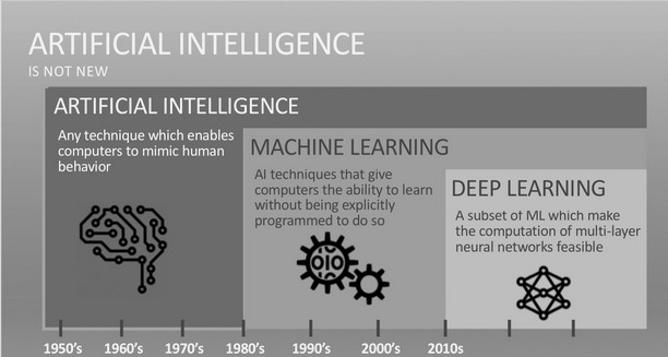
Theory Behind NNs
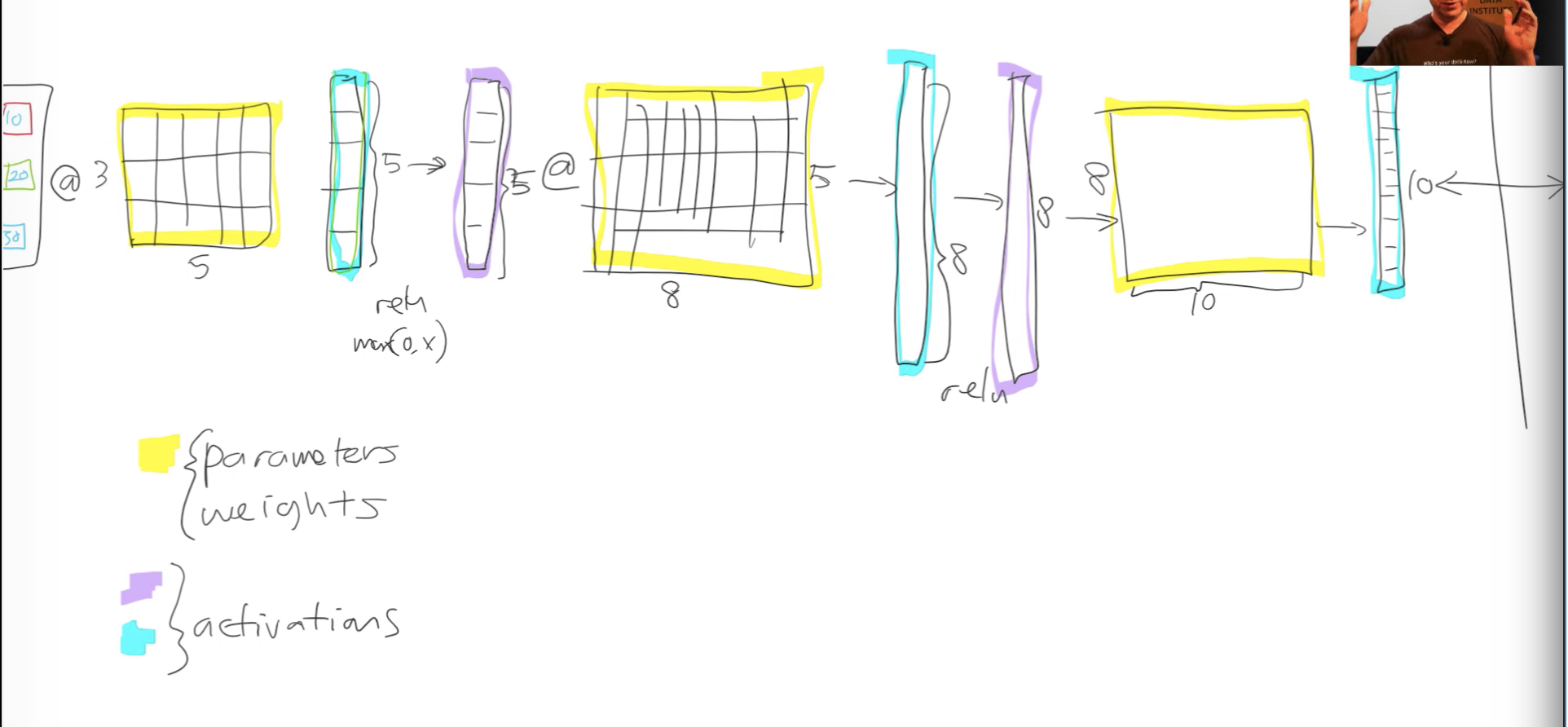
Dataloaders -> [ Linear Function (Matrix Multiplication) -> Activation Function] -> Next layer …
Back propagation is nothing but
parameters minus= learning rate * parameters.gradient_descent(loss function) i.e.
parameters = parameters minus learning rate * parameters.gradient_descent(loss function)
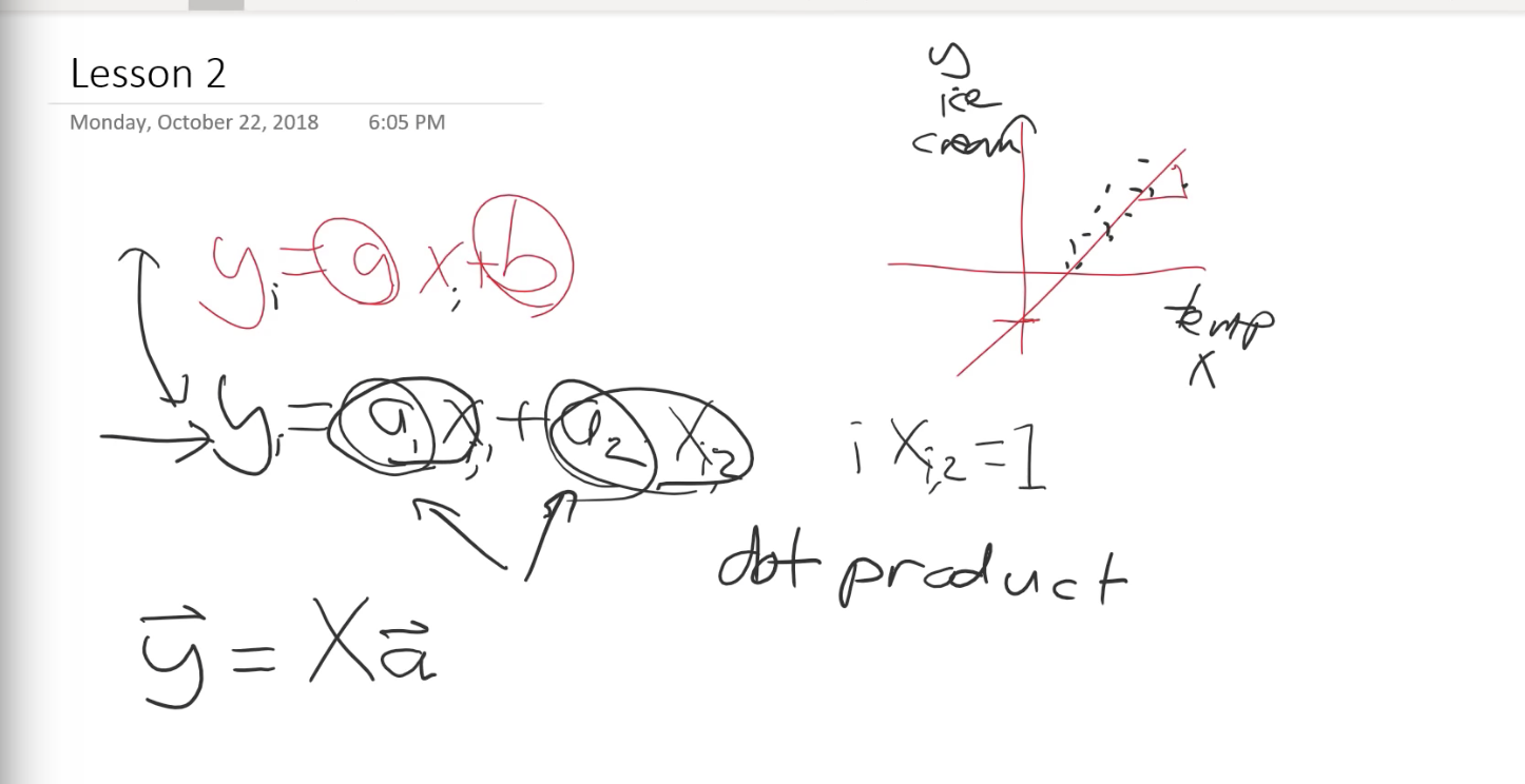
Revision of GD (Gradient Descent) (Lesson 2 from the middle of the video)
Yi= a1Xi1+a2Xi2+constant and let’s assume Xi2=1 for simplicity.
If the above equation is executed for different “i” it will become a matrix multiplication.
Using pytorch above equation can be written as below. (X first column is Random numbers)
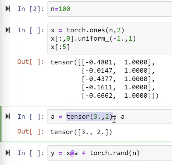
Tensor is a regular sized (non-ragged) array. It can be rectangular (2D) or a Cube (3D) or more dimensions. But it is always a regular size.
An example – Image is a Rank 3 tensor since it has 3 layers (RGB).
If we plot the y function from screenshot above
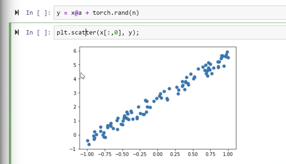
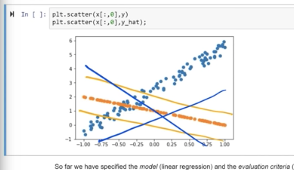
If we want to fit a line through these points without knowing the coefficients 3 and 2 i.e. Tensor A, we start with some random values and we can plot the line.
We can move around the line by using the derivative of the Loss (in this case MSE) and see how Y changes.
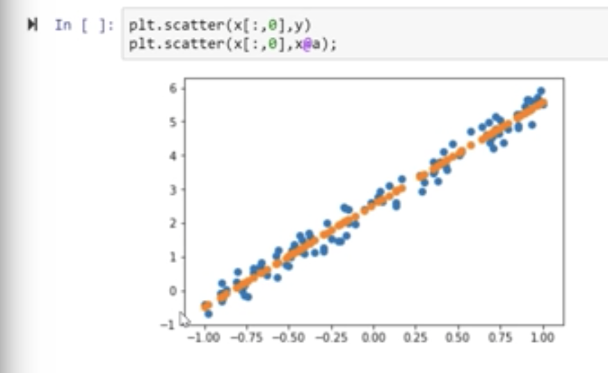
MSE – (y_hat(prediction)-y(actual))**2.mean()
Loss is nothing but the distance of the line from the dots. If we reduce the loss, the line will match the dots and go through them thereby keeping the loss at a minimum.
The gradient/derivative is used along with learning rate to change the value of the co-efficients and bring the line closer to where we want.
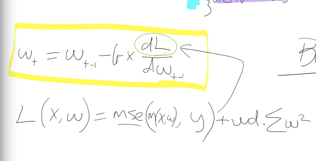
Weight Decay – All learners have a weight decay parameters in fastai and a value of 0.1 should help in general.
W- Weights/Parameters
L(x,w) – Loss function
M(x,w) – y_hat
The box is same as
parameters = parameters minus learning rate * parameters.gradient_descent(loss function)
Momentum – The update to the parameters/weights is not just based on the derivative, instead 1/10 of it is the derivative and 90% of it is just the same direction that we went last time. This is exponentially weighted moving average of the step.
Generally, a momentum of 0.9 is used with SGD if we want to use momentum.
RMSProp – This is similar to Momentum but it is exponentially weighted moving average of the gradient squared.
Adam is Momentum + RMSProp – https://github.com/hiromis/notes/blob/master/Lesson5.md
Cross Entropy Loss – Loss used for Single Label Multi class classification problem
SoftMax Activation function – Activation function used in Single Label Multi class classification problems.
RESNET – Residual Net. The input from previous layer is added to this layer’s output. In other words the inputs skips this convolution (skip connection). Added is a + here. This is the basic theory of Resnet.
DenseNet – Same as resnet but instead of a +, a concat is used to concatenate previous layer’s input and its output and that is passed to this layer. It is memory intensive but works well for smaller datasets.
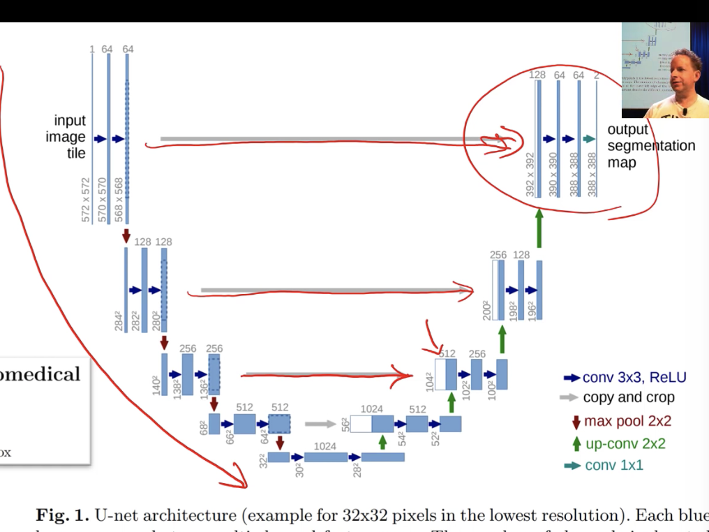
UNet – As the name says, it is in a U shape. It can be thought of Resnet from halfpoint onwards.
Example - First layer output is skipping all layers and directly going as input to last layer.
Nearest Neighbor interpolation
Bi Linear interpolation – In layman terms - Techniques to increase the resolution sizes of image inputs.
CNN –
The matrix multiplications in a NN are replaced with a special Matrix multiplication in case of CNNs and they are called Convolutions.
Conv Kernel multiplied by Input matrix to get one single number. Kernel Matrix can be considered to be a matrix of weights which are tied at certain places and also is sparse.
By doing this, we achieve identifying different parts of an image and later it can all be tied together to identify the whole image.
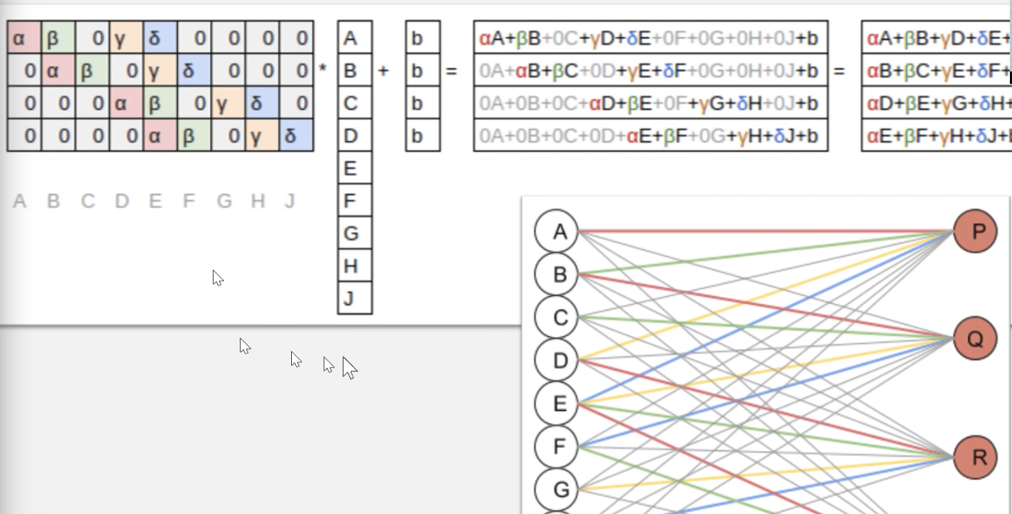
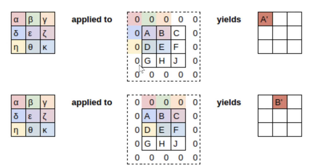
For example – a 3x3 matrix multiplied to another 3x3 gives a 3x3 in normal matrix multiplication. However, convolution will only give a single value.
Therefore, it is generally padded with zeroes to as shown below.
Note : This is 2D example, However images are generally 3D and the same idea extends to that as well. You will have more conv kernels and so on. For images, it could be 3 conv kernels to start with along with some kind of padding to increase the size of the Tensor. However practically, there are more kernels used even during start.
However, we don’t use Matrix multiplication since its slow and the matrix is anyways sparse with many zeroes.
There are functions which do this called Convolution functions.
Stride 2 Convolution – Same as above, but skip one layer of cells or columns in matrix when moving to next section. After the left top corner is done, you skip to top right corner in above example instead of the middle 3 columns. This reduces the height and width of output matrix but we generally increase the kernels and the depth (channels) actually increases.
Average Pooling – After multiple layers, we will have more number of channels and some small height and width. What we need is Category of the image in a Image classifier. There could be say 5 categories. To get to this point, we do various things and one of the first things is Average pooling. It basically takes average of each channel. If the final layer gave an output of say 20 layers, we take average of each layer and get one value for each layer. These are stacked in a column vector of size 20. This is still more than the categories we expect.
This is passed through a linear layer to get the 5 categories that we want. One of the categories in this vector should have a high probability value based on which the prediction can be obtained.
ResNet – See above.
DenseNet – See above.
UNET – See above.
UNET gives an output image of same size as input. The down sampling reduces the image size for sure and we know that. For increasing the size by final layer, it does a Stride ½ convolution.
Apart from padding on the perimeter, it also adds padding in between as shown below.
The 2x2 blue colored pixels are original image. Remaining are all padding.
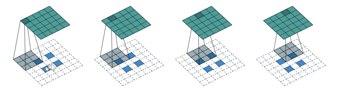
This is slightly older where all the padded pixels are basically zeros or white pixels.
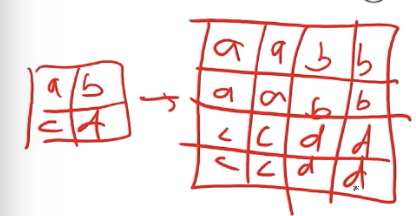
Below is what is done now to do up-sampling. This is called Nearest Neighbor interpolation.
Bilinear Interpolation is similar but takes a weighted average of the surrounding neighbors.
Techniques like above are used in up sampling path of the UNET. However the down sampling would have reduced the size and up sampling only from that will be not useful.
A skip connection or identity connection is added in up direction where the inputs of the down sampling path are added as inputs. See UNET diagram above.
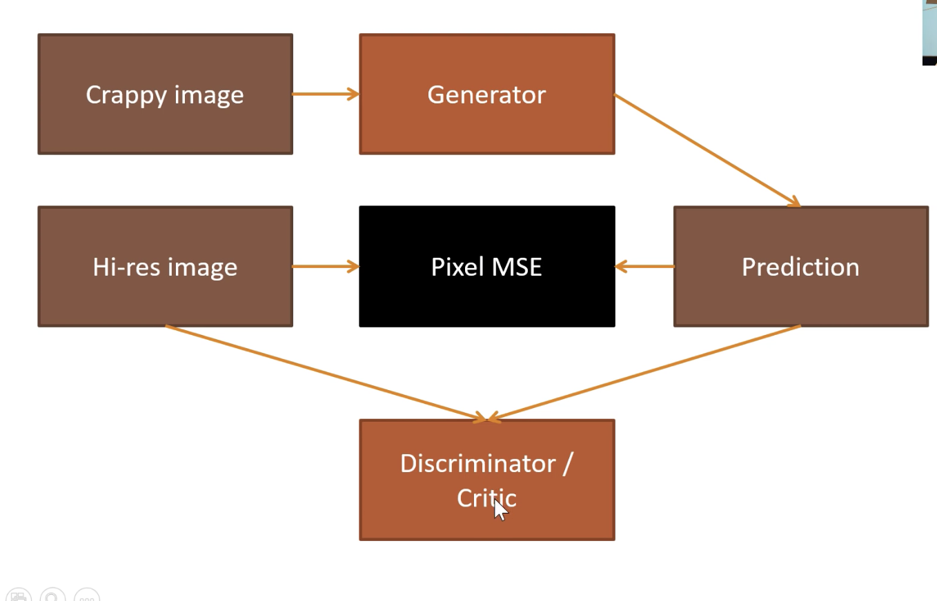
GAN
RNN
-
Inputs – Get the inputs as Tensors
-
Weights/Parameters/Coefficients – Multiply with Random weights or Pretrained weights. This is Linear computation i.e. Linear layer or Affine Layer.
-
Activations – The output of Affine function are also Activations. But they are Linear activations. Pass the output of previous step through a non linear activation function like ReLU or Softmax. This is the non-linearity in the NeuralNet.
- Activation Function – ReLU, Softmax, Sigmoid and many others.
-
Output – The output is obtained.
-
Layers – Each of these is a layer
-
Loss – Compare the output with actual output and calculate the Loss. MSE, RMSE, Log(MSE) etc are some of the Loss functions.
L(x,w) = MSE(m(x,w),y) +WD* Sum(W**2)
Since we calculate the gradient of a Loss function, that calculates the gradient of the WD*(Sum(W**2))
Adding the +WD* Sum(W**2) to Loss function is called L2 regularization.
The gradient of WD*(Sum(W**2)) which is used in Back propagation (params = params-LR*gradient (Loss function) i.e. 2*WD*W (generalized to WD*W) is called Weight Decay.
-
Back propagation is nothing but parameters = parameters minus learning rate * parameters.gradient_descent(loss function)
-
One Hot Encoded Matrix – This is done to preprocess the input data that is fed to a neural net. This is helpful to pass the data into NN in a common format of Matrices. One matrix of One Hot Encoded Matrix and the other input Random Weights Matrix.
-
Embedding – Array Lookup or Matrix Multiply by One hot encoded matrix.
-
Latent features or Latent Factors – Insights that NNs can give. Embeddings also give latent features in Collab learning.
-
N_factors in collab problems - Size of the embedding matrix.
-
Weight Decay - Weight Decay is a type of Regularization. Weight decay is a number used to multiply the parameters during Loss calculation. We should use many parameters and along with that use weight decay. General value should be 0.1
Parameters at time/epoch T = parameters at epoch T-1 – LR*derivative (loss with respect to parameters at T-1)
-
Adam – Momentum+RMS Prop
-
Momentum - parameters = parameters minus learning rate * [ x% (parameters.gradient_descent(loss function)) + (100-x)% (previous derivative)]
- Or it can also be written as Step T = alpha*gradient + (1-alpha)*Step T-1 . This second part of 1-alpha is called Exponentially weighted moving average of past gradients. Step T-1 inturn uses Step T-2. So (1-alpha) gets multiplied multiple times.
-
RMS Prop - Exponentially weighted moving average of past gradient square and use that to divide as shown below
-
parameters = parameters minus learning rate *{ [ x% (parameters.gradient_descent(loss function)) + (100-x)% (previous derivative)]}/{ Exponentially weighted moving average of past gradient square}
-
Metric
-
User Bias and Item Bias – Terms in Collab which highlight the biases that the user (like customer id, user_id) can have and the biases of the Item (like movie (popular movie) or product (star product like Apple devices))
-
Cross-Entropy – Loss function where we want a single value to be selected as output rather than probability of being close to the output. That is why it’s used in Single Label Multi class classification problems.
-
Loss cannot be MSE for learners which predict individual classes. MSE is more suited for finding a number on a graph kinda problems.
-
Cross Entropy is a Loss function which provides low loss when the prediction is correct and its confident and high loss for wrong predictions with high confidence.
-
-
Softmax – For Cross Entropy Loss function to work correctly and give positive probability and to be sure that sum of probabilities for possible values to be less than 1, the activation function to be used along with this Loss function is Softmax function.
-
Dropout – Dropout is a type of regularization. Some activations are thrown out in each mini batch. We keep lot of parameters but throw away some activation randomly in each mini batch so that it does not overfit.
-
BatchNorm – Generally for continuous variables. Used for most cases. This is basically to scale up the output. For example if the range of values we expect is 1 to 5, but the NN gives -1 to 1, using batch norm layer would help to normalize it..
-
Yhat = f(w0, w1, w2…. Wn, X)*g + b
-
Loss = Sum (y-yhat)**2
-
-
WeightNorm is another new normalization used in Fastai. Recent thing..
-
Data Augmentation - Modify model inputs during training in order to effectively increase data size. For examples - Images can be flipped or warped or perspective changes etc to basically convert one image into multiple images which look different from one another.
-
Label_Cls option in Tabular - Used to pass options like Output variable to be considered a Float, Take Log of it while creating labels for it etc..
-
Tabular Architecture - Mostly Embeddings of many layers.
-
Data Augmentation
-
Fine Tuning
-
Layer Deletion and Random weights
-
Freezing and Unfreezing